【RayTracer】（二）实现物体类

有了基本工具类，现在我们可以回顾图形学中的知识，从最简单的渲染一个球体开始，逐渐熟悉光线追踪的实现。

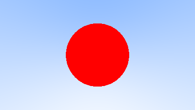
1 渲染一个球体

在光线追踪中如果投射出的光线碰到了物体，就计算该点的颜色作为像素值，那么我们从最简单的情形开始，渲染一个球体，我们在 z = -1 处放置一个球体，然后计算投射出的每一条光线和该球体是否有交点，如果有的话我们将该像素设置为一个定值，这样就可以在屏幕上显示出这个球体了。

计算光线和空间中球体是否有交点我们在图形学中已经学过，非常简单，对于射线 $P(t)$ 和一个空间中球心在 $C$ ，半径为 $r$ 的球体，如果射线上的点在球面上，则满足：
$$
(P(t)−C)⋅(P(t)−C)=r^2
$$
将 $P(t) = A + t \vec b$ 代入得：
$$
(A+t\vec b−C)⋅(A+t\vec b−C)=r^2
$$
再展开即可得到关于 $t$ 的一元二次方程：
$$
t^2 \vec b⋅\vec b+2t\vec b⋅(A−C)+(A−C)⋅(A−C)−r^2=0
$$
只需要判断这个一元二次方程有没有实数根即可。于是我们可以写出判断光线是否和球体相交的函数：

// 判断光线是否与球体相交
bool hit_sphere(const point3& center, double radius, ray& r) {
	vec3 oc = r.origin() - center;
	auto a = dot(r.direction(), r.direction());
	auto b = 2.0 * dot(oc, r.direction());
	auto c = dot(oc, oc) - radius * radius;
	auto discriminant = b * b - 4 * a * c;
	return (discriminant > 0);
}

然后在之前的 ray_color 函数中加上判断光线是否和球体相交的代码：

// 得到光线颜色
color ray_color(ray& r)
{
	//放置在 z = -1 处的一个半径为0.5的球体
	if (hit_sphere(point3(0, 0, -1), 0.5, r)) return color(1, 0, 0);
	vec3 unit_dir = normalize(r.direction());
	// 归一化后y的范围是[-1,1]，将其映射到[0,1]作为混合系数
	auto t = 0.5 * (unit_dir.y() + 1.0);
	return (1.0 - t) * color(1.0, 1.0, 1.0) + t * color(0.5, 0.7, 1.0);
}

效果如下：

需要注意的是，现在我们只考虑了是否有实数根，并没有考虑 t 的正负，这会导致即使把球体放到 z = 1 处，也能得到和上图相同的结果，这相当于我们看到了在相机后面的物体，这个问题之后我们会解决。

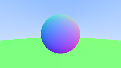
2 表面法线

2.1 可视化物体表面法线

我们计算光线与物体交点的光照时首先需要知道该交点的法线，对于一个球体来说，表面上任意一点的法线方向就是该点和球心连线的方向并从球心向外指。因此我们只要计算出投射的光线和球体的交点就可以得到该点的法向量，由于法向量是单位向量，每个分量范围都在 [-1, 1] ，因此我们可以将每个分量都映射到 [0, 1]，作为颜色值显示出来。

为此我们先修改刚才的 hit_sphere 使其返回交点的 t 值，由于我们的球体放在 z = -1 处，所以两个交点都一定是正实数，我们返回较小的那个一根即可，即：
$$
t_{return} = \frac{-b - \sqrt{b^2-4ac} }{2a}
$$
因为只能看到离我们最近的点，修改后的代码如下：

// 判断光线是否与球体相交
double hit_sphere(const point3& center, double radius, ray& r) {
	vec3 oc = r.origin() - center;
	auto a = dot(r.direction(), r.direction());
	auto b = 2.0 * dot(oc, r.direction());
	auto c = dot(oc, oc) - radius * radius;
	auto discriminant = b * b - 4 * a * c;
	if (discriminant < 0) {
		return -1.0;
	}
	else {
		return (-b - sqrt(discriminant)) / (2.0 * a);
	}
}

同时修改 ray_color 函数：

// 得到光线颜色
color ray_color(ray& r)
{
	//放置在 z = -1 处的一个半径为0.5的球体，计算交点法线作为颜色返回
	auto t = hit_sphere(point3(0, 0, -1), 0.5, r);
	if (t > 0)
	{
		vec3 normal = normalize(r.at(t) - vec3(0, 0, -1));
		return (normal + vec3(1, 1, 1)) * 0.5;
	}
	vec3 unit_dir = normalize(r.direction());
	// 归一化后y的范围是[-1,1]，将其映射到[0,1]作为混合系数
	t = 0.5 * (unit_dir.y() + 1.0);
	return (1.0 - t) * color(1.0, 1.0, 1.0) + t * color(0.5, 0.7, 1.0);
}

渲染效果如下：

2.2 代码优化

上面的 hit_sphere 函数有一些可以优化的地方，首先两个相同向量的点乘，可以通过我们在 vec3 类中定义的 length_squared() 方法得到，另外考虑方程的求根公式：
$$
\frac{-b \pm \sqrt{b^2-4ac} }{2a}
$$
如果把 b 替换成 2h，可以得到：
$$
\frac{-2h \pm \sqrt{(2h)^2-4ac} }{2a}
$$
展开整理得：
$$
\frac{-h \pm \sqrt{h^2-ac} }{a}
$$
于是我们只需要计算 b 的一半即可：

// 判断光线是否与球体相交
double hit_sphere(const point3& center, double radius, ray& r) {
	vec3 oc = r.origin() - center;
	auto a = r.direction().length_squared();
	auto h = dot(oc, r.direction());
	auto c = dot(oc, oc) - radius * radius;
	auto discriminant = h * h - a * c;
	if (discriminant < 0) {
		return -1.0;
	}
	else {
		return (-h - sqrt(discriminant)) / a;
	}
}

3 多个物体

3.1 实现物体类

在实际场景中我们不可能只有一个物体，并且物体也不可能只是球体，还可能有有各种各样的模型，因此为了能让所有模型都可以放置到场景中并计算我们投射光线和物体的交点，我们可以先定义一个可计算交点的抽象物体类 hittable，这个类定义一个纯虚函数 hit 用来判断物体和光线的交点，然后再以该抽象类为基类，实现各种物体类即可，这样一来，不同的物体的 hit 函数有可以有不同的实现了。

hit 函数也和我们上面写的稍有不同，除了要接收一根光线作为参数外，还要有一个限定范围 $t_{min}$ 和 $t_{max}$，只有当交点的 t 在这个范围内才会与物体相交，这部分也在之前的图形学中也有学过，同时这个范围也可以用于后面计算多个物体中最近的交点。

此外，光线可能和物体有多个交点，我们需要取在限定范围内的离我们最近的交点，把该交点及其法线等属性记录下来，因此还要定义一个存储交点属性的结构体。

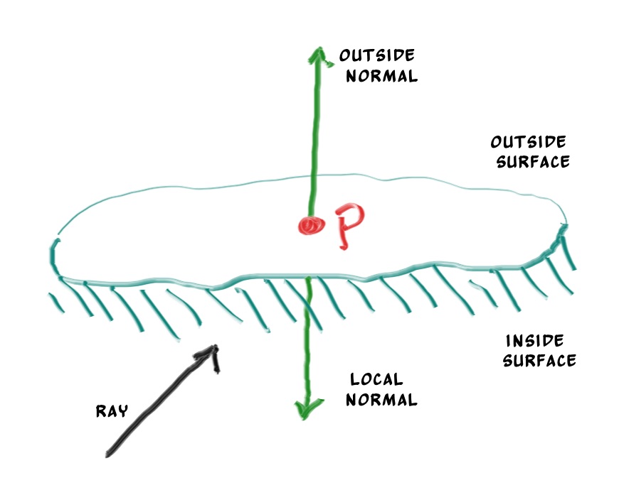
最后还需要考虑一个问题，交点是物体的正面还是背面？这对我们渲染来说非常重要，尤其是一些双面不同的物体。这可以通过光线和法线的点乘来判断，如果光线和交点的法线反向，这说明交点在物体的正面，因为法线都是从物体中心指向表面的；相反如果光线和交点的法线同向，这说明交点在物体的背面。同向和反向实际上是两个向量的夹角，因此点乘即可。如果交点在物体背面，那么计算光照时用到的法线应该是这个点表面法线的反方向，所以要对原法线取反。如下图：

现在我们可以开始实现上面的思路了，首先是抽象类和结构体的定义：

/*
    抽象类hittable，所有物体都继承该类
*/
#pragma once
#ifndef HITTABLE_H
#define HITTABLE_H
// utilities.h 包含了常用的工具函数并整合了常用头文件，避免循环嵌套，我们在后面会实现
#include "utilities.h"

struct hit_record {
    point3 p;           //交点
    vec3 normal;        //交点法线
    double t;           //交点t值
    bool front_face;    //交点是否在物体的正面
    // 如果交点在物体的背面，则法线应该取反方向，以用于计算光照
    inline void set_face_normal(ray& r, vec3& outward_normal) {
        front_face = dot(r.direction(), outward_normal) < 0;
        normal = front_face ? outward_normal : -outward_normal;
    }
};

class hittable {
public:
    // 纯虚函数，在派生类中实现
    virtual bool hit(ray& r, double t_min, double t_max, hit_record& rec) const = 0;
};

#endif

接下来实现一个球体类：

/*
    球体类sphere，派生于基类hittable
*/
#pragma once
#ifndef SPHERE_H
#define SPHERE_H

#include "hittable.h"

// 球体类以hittable抽象类为基类
class sphere : public hittable {
public:
    sphere() {}
    sphere(point3 cen, double r) : center(cen), radius(r) {};
    // 重载虚函数
    virtual bool hit(ray& r, double t_min, double t_max, hit_record& rec) const override;

public:
    point3 center;
    double radius;
};

bool sphere::hit(ray& r, double t_min, double t_max, hit_record& rec) const
{
    vec3 oc = r.origin() - center;
    auto a = r.direction().length_squared();
    auto half_b = dot(oc, r.direction());
    auto c = oc.length_squared() - radius * radius;

    auto discriminant = half_b * half_b - a * c;
    if (discriminant < 0) return false;
    auto sqrtd = sqrt(discriminant);

    // 找到满足条件的最近的交点
    auto root = (-half_b - sqrtd) / a;
    if (root < t_min || t_max < root) {
        root = (-half_b + sqrtd) / a;
        if (root < t_min || t_max < root)
            return false;
    }
    // 记录该交点的相关信息
    rec.t = root;
    rec.p = r.at(rec.t);
    // 法线记得归一化
    vec3 outward_normal = (rec.p - center) / radius;
    // 判断交点在正面还是背面，并设置正确的法线方向
    rec.set_face_normal(r, outward_normal);

    return true;
};

#endif

3.2 实现物体列表类

现在我们已经有了可以与光线相交的物体的基类 hittable，可以在其基础上实现各种物体类，接下来我们要定义一个类来存储多个物体，代码比较容易理解：

/*
	物体列表类hittable_list
*/
#pragma once
#ifndef HITTABLE_LIST_H
#define HITTABLE_LIST_H

#include "hittable.h"
#include <memory>
#include <vector>

using std::shared_ptr;
using std::make_shared;

class hittable_list : public hittable {
public:
    hittable_list() {}
    hittable_list(shared_ptr<hittable> object) { add(object); }

    void clear() { objects.clear(); }
    void add(shared_ptr<hittable> object) { objects.push_back(object); }
    // 一个物体列表的hit函数用于得到光线和这个列表中所有物体最近的一个交点
    virtual bool hit(ray& r, double t_min, double t_max, hit_record& rec) const override;

public:
    std::vector<shared_ptr<hittable>> objects;
};

bool hittable_list::hit(ray& r, double t_min, double t_max, hit_record& rec) const
{
    hit_record temp_rec;
    bool hit_anything = false;
    // 记录当前的最近的t
    auto closest_so_far = t_max;
    // 遍历每一个物体
    for (const auto& object : objects) {
        if (object->hit(r, t_min, closest_so_far, temp_rec)) {
            hit_anything = true;
            // 更新最近的t
            closest_so_far = temp_rec.t;
            rec = temp_rec;
        }
    }

    return hit_anything;
}

#endif

3.3 关于智能指针

上面的物体列表类中使用了智能指针，在之后的代码中我们也会经常使用，智能指针能帮助我们自动管理内存，防止内存泄漏，一般来说初始化一个智能指针可以使用如下形式的代码：

shared_ptr<double> double_ptr = make_shared<double>(0.37);
shared_ptr<vec3>   vec3_ptr   = make_shared<vec3>(1.414214, 2.718281, 1.618034);
shared_ptr<sphere> sphere_ptr = make_shared<sphere>(point3(0,0,0), 1.0);

auto 支持对智能指针类型的自动推导，因此我们写起来会更方便：

auto double_ptr = make_shared<double>(0.37);
auto vec3_ptr   = make_shared<vec3>(1.414214, 2.718281, 1.618034);
auto sphere_ptr = make_shared<sphere>(point3(0,0,0), 1.0);

声明后就可以像正常指针一样使用了。更多关于智能指针的内容可以查看 C++ 与 STL 部分的笔记。

4 常用常量和工具函数

接下来需要定义一些常用的常量以及角度转弧度等工具函数，并将一些类的头文件整合起来，使代码组织更整洁。

/*
	常用常量及工具函数
	整合包含其他头文件
*/
#pragma once

#ifndef UTILITIES_H
#define UTILITIES_H

#include <cmath>
#include <limits>
#include <memory>

using std::shared_ptr;
using std::make_shared;
using std::sqrt;

// 常量
const double infinity = std::numeric_limits<double>::infinity();
const double pi = 3.1415926535897932385;

// 工具函数
inline double degrees_to_radians(double degrees) {
	return degrees * pi / 180.0;
}

// 常用头文件

#include "ray.h"
#include "vec3.h"

#endif UTILITIES_H

5 再次可视化法线

使用上面实现的一系列代码，再次实现一个可视化法线的效果，首先修改 ray_color 函数：

// 得到光线颜色
color ray_color(ray& r, const hittable& world) {
	hit_record rec;
	// 计算和世界中的物体的交点的法线
	if (world.hit(r, 0, infinity, rec)) {
		return 0.5 * (rec.normal + color(1, 1, 1));
	}
	vec3 unit_direction = normalize(r.direction());
	auto t = 0.5 * (unit_direction.y() + 1.0);
	return (1.0 - t) * color(1.0, 1.0, 1.0) + t * color(0.5, 0.7, 1.0);
}

然后是主函数：

#include <iostream>
#include <string>
#include "utilities.h"
#define STB_IMAGE_WRITE_IMPLEMENTATION
#include "stb_image_write.h"
#include "hittable_list.h"
#include "sphere.h"
#include "color.h"

int main()
{
    /****图片保存，保存为png格式****/
    std::string SavePath = "D:\\TechStack\\ComputerGraphics\\Ray Tracing in One Weekend Series\\Results\\";
    std::string filename = "WorldSphereNormal.png";
    std::string filepath = SavePath + filename;
    
    /*******图片属性*******/ 
    // 宽高比
    const auto aspect_ratio = 16.0 / 9.0;
    const int image_width = 400;
    // 使用static_cast可以明确告诉编译器，这种损失精度的转换是在知情的情况下进行的
    // 也可以让阅读程序的其他程序员明确你转换的目的而不是由于疏忽
    const int image_height = static_cast<int>(image_width / aspect_ratio);
    const int channel = 3;

    /*******相机属性*******/
    // 视口高度设为两个单位
    auto viewport_height = 2.0;
    // 视口宽度根据屏幕宽高比计算
    auto viewport_width = aspect_ratio * viewport_height;
    // 原点到视口平面距离为1个单位
    auto focal_length = 1.0;
    // 相机原点
    auto origin = point3(0, 0, 0);
    // 视口宽的一半
    auto horizontal = vec3(viewport_width, 0, 0);
    // 视口高的一半
    auto vertical = vec3(0, viewport_height, 0);
    // 相当于将(0,0,0)移动到视口平面的左下角，也就是得到左下角的点的位置
    auto lower_left_corner = origin - horizontal / 2 - vertical / 2 - vec3(0, 0, focal_length);

    /*******场景属性*******/
    hittable_list world;
    // 向场景中添加两个球体
    world.add(make_shared<sphere>(point3(0, 0, -1), 0.5));
    world.add(make_shared<sphere>(point3(0, -100.5, -1), 100));

    /******渲染部分*****/
    // 3通道图像存在一维数组中
    unsigned char* odata = (unsigned char*)malloc(image_width * image_height * channel);
    unsigned char* p = odata;
    for (int j = image_height - 1; j >= 0; --j) {
        // 标准错误流显示进度信息，单行刷新显示
        std::cerr << "\rScanlines remaining: " << j << ' ' << std::flush;
        for (int i = 0; i < image_width; ++i) {
            // x方向偏移
            auto u = double(i) / (image_width - 1);
            // y方向偏移
            auto v = double(j) / (image_height - 1);
            ray r(origin, lower_left_corner + u * horizontal + v * vertical - origin);
            color pixel_color = ray_color(r, world);
            write_color(p, pixel_color);
        }
    }
    stbi_write_png(filepath.c_str(), image_width, image_height, channel, odata, 0);
    std::cerr << "\nDone.\n";
}

渲染效果如下：